Getting started
A quick overview of FLEXPART data
reflexible was originally developed for working with FLEXPART V8.x which has some fairly new features to how the output data is created. The latest version of FLEXPART also has functionality for saving directly to Netcdf. The ability to read this data directly is forthcoming, but for now reflexible still only works with the raw unformatted binary Fortran data FLEXPART has traditionally used for output. See the documents for information regarding FLEXPART .
A users guide for FLEXPART is available which explains the model output.
Note If you are interested in contributing functionality for other FLEXPART versions, please contact me.
reflexible was originally released as ‘pflexpart’, but as the goal is to be more generic, the package was renamed. The current release is still focused on FLEXPART, but some generalizations are starting to make their way into the code base.
reflexible is undergoing constant modifications and is not particularly stable or backward compatible code. I am trying to move in the right direction, and have moved the code now to github.org. If you are interested in contributing, feel free to contact me: John F. Burkhart
Fetching example data
An example data set is available for testing. The data contains a backward run case from Svalbard, and is suitable for testing some of the unique functions of reflexible for analysis and creation of the retroplumes.
I suggest using wget to grab the data:
$ wget http://folk.uio.no/johnbur/sharing/stads2_V10.tar
Converting FLEXPART output to netCDF4 format
Reflexible is using a netCDF4 internally for doing its analysis and plotting duties. This section demonstrates how to convert the FLEXPART output to netCDF4 format. In order to do that the create_ncfile script will be invoked. This script is copied into a directory in your path when reflexible is installed, so you should not worry about copying it manually.
Before processing the data in stads2_V10.tar we have to uncompress that file:
$ cp stads2_V10.tar /tmp
$ cd /tmp
$ tar xvf stads2_V10.tar
After untarring, a directory named stads2_V10 is created. It contains the result of processing a simple backward run case with FLEXPART. Next we can execute the fprun script:
$ fprun /tmp/stads2_V10/pathnames
Flexpart('/tmp/stads2_V10/pathnames', nested=False)
note that you pass the pathnames of a FLEXPART run. The pathnames file has a simple structure. For example, in our case it goes like this:
$./options/
./stads2_15_018.001/
/
/.../AVAILABLE_ECMWF_OPER_fields_global
============================================
So, basically in the first line indicates the <options> directory for the FLEXPART run, whereas the second line specifies the <output> directory. With this, you can easily mix and match different <options> and <output> directories for your analysis.
If we want to select the nested data instead, just pass the -n flag:
$ fprun -n /tmp/stads2_V10/pathnames
Flexpart('/tmp/stads2_V10/pathnames', nested=True)
And if you want to get some info on the COMMANDS file:
$ fprun -n -C /tmp/stads2_V10/pathnames
$ Flexpart('/tmp/stads2_V10/pathnames', nested=True)
$ Command: OrderedDict([('CBLFLAG', 0), ('CTL', -5), ('IBDATE', 20150405), ('IBTIME', 103500), ('IEDATE', 20150426), ('IETIME', 130500), ('IFINE', 4), ('IFLUX', 0), ('IND_RECEPTOR', 1), ('IND_SOURCE', 1), ('IOUT', 13), ('IOUTPUTFOREACHRELEASE', 1), ('IPIN', 0), ('IPOUT', 0), ('ITSPLIT', 9999999), ('LAGESPECTRA', 1), ('LCONVECTION', 1), ('LDIRECT', -1), ('LINIT_COND', 0), ('LOUTAVER', 10800), ('LOUTSAMPLE', 900), ('LOUTSTEP', 10800), ('LSUBGRID', 1), ('LSYNCTIME', 900), ('MDOMAINFILL', 0), ('MQUASILAG', 0), ('NESTED_OUTPUT', 1), ('SURF_ONLY', 0)])
You can get more info on the supported flags by passing the -h flag to the fprun command line utility:
$ fprun -h
usage: fprun [-h] [-n] [-C] [-R] [-S] [-H HEADER_KEY] [-K] [pathnames]

positional arguments:
  pathnames             The Flexpart pathnames file stating where options and
                        output are. If you pass a dir, a 'pathnames' file will
                        be appended automatically. If not found yet, a FP
                        output dir is assumed.

optional arguments:
  -h, --help            show this help message and exit
  -n, --nested          Use a nested output.
  -C, --command         Print the COMMAND contents.
  -R, --releases        Print the RELEASES contents.
  -S, --species         Print the SPECIES contents.
  -H HEADER_KEY, --header-key HEADER_KEY
                        Print the contents of H[HEADER_KEY].
  -K, --header-keys     Print all the HEADER keys.
Reading data out of a FLEXPART run
Newer versions of FLEXPART can generate convenient NetCDF4 files as output, so let’s have a quick glimpse on how you can access the different data on it.
Note In case you have a FLEXPART output that is not in NetCDF4 format, you can always make use the create_ncfile command line utility.
Open the file and print meta-information for the run:
In [1]: from netCDF4 import Dataset

In [2]: rootgrp = Dataset("/tmp/stads2_V10/stads2_15_018.001/grid_time_20150426130500.nc")

In [3]: print(rootgrp)
<class 'netCDF4._netCDF4.Dataset'>
root group (NETCDF4 data model, file format HDF5):
    Conventions: CF-1.6
    title: FLEXPART model output
    institution: NILU
    source: Version 10.0beta (2015-05-01) model output
    history: 2016-02-02 09:43 +0100  created by  on compute-8-16.local
    references: Stohl et al., Atmos. Chem. Phys., 2005, doi:10.5194/acp-5-2461-200
    outlon0: -179.0
    outlat0: -90.0
    dxout: 0.5
    dyout: 0.5
    ldirect: -1
    ibdate: 20150405
    ibtime: 103500
    iedate: 20150426
    ietime: 130500
    loutstep: -10800
    loutaver: -10800
    loutsample: -900
    itsplit: 9999999
    lsynctime: -900
    ctl: -0.2
    ifine: 1
    iout: 5
    ipout: 0
    lsubgrid: 1
    lconvection: 1
    lagespectra: 1
    ipin: 0
    ioutputforeachrelease: 1
    iflux: 0
    mdomainfill: 0
    ind_source: 1
    ind_receptor: 1
    mquasilag: 0
    nested_output: 1
    surf_only: 0
    linit_cond: 0
    dimensions(sizes): time(168), longitude(720), latitude(360), height(3), numspec(1), pointspec(31), nageclass(1), nchar(45), numpoint(31)
    variables(dimensions): int32 time(time), float32 longitude(longitude), float32 latitude(latitude), float32 height(height), |S1 RELCOM(numpoint,nchar), float32 RELLNG1(numpoint), float32 RELLNG2(numpoint), float32 RELLAT1(numpoint), float32 RELLAT2(numpoint), float32 RELZZ1(numpoint), float32 RELZZ2(numpoint), int32 RELKINDZ(numpoint), int32 RELSTART(numpoint), int32 RELEND(numpoint), int32 RELPART(numpoint), float32 RELXMASS(numspec,numpoint), int32 LAGE(nageclass), int32 ORO(latitude,longitude), float32 spec001_mr(nageclass,pointspec,time,height,latitude,longitude)
    groups:
We can get the info for a specific attribute just by referencing it like this:
In [4]: print(rootgrp.loutstep)
-10800
We can have a look at the different dimensions and variables in the file:
In [5]: print(rootgrp.dimensions)
OrderedDict([('time', <class 'netCDF4._netCDF4.Dimension'> (unlimited): name = 'time', size = 168
), ('longitude', <class 'netCDF4._netCDF4.Dimension'>: name = 'longitude', size = 720
), ('latitude', <class 'netCDF4._netCDF4.Dimension'>: name = 'latitude', size = 360
), ('height', <class 'netCDF4._netCDF4.Dimension'>: name = 'height', size = 3
), ('numspec', <class 'netCDF4._netCDF4.Dimension'>: name = 'numspec', size = 1
), ('pointspec', <class 'netCDF4._netCDF4.Dimension'>: name = 'pointspec', size = 31
), ('nageclass', <class 'netCDF4._netCDF4.Dimension'>: name = 'nageclass', size = 1
), ('nchar', <class 'netCDF4._netCDF4.Dimension'>: name = 'nchar', size = 45
), ('numpoint', <class 'netCDF4._netCDF4.Dimension'>: name = 'numpoint', size = 31
)])

In [6]: rootgrp.variables.keys()
Out[11]: odict_keys(['time', 'longitude', 'latitude', 'height', 'RELCOM', 'RELLNG1', 'RELLNG2', 'RELLAT1', 'RELLAT2', 'RELZZ1', 'RELZZ2', 'RELKINDZ', 'RELSTART', 'RELEND', 'RELPART', 'RELXMASS', 'LAGE', 'ORO', 'spec001_mr'])
The netCDF4 Python wrappers allows to easily slice and dice variables:
In [15]: longitude = rootgrp.variables['longitude']

In [16]: print(longitude)
<class 'netCDF4._netCDF4.Variable'>
float32 longitude(longitude)
    long_name: longitude in degree east
    axis: Lon
    units: degrees_east
    standard_name: grid_longitude
    description: grid cell centers
unlimited dimensions:
current shape = (720,)
filling on, default _FillValue of 9.969209968386869e+36 used
We see that ‘longitude’ is a unidimensional variable with shape (720,). Let’s read just the 10 first elements:
In [20]: longitude[:10]
Out[20]:
array([-178.75, -178.25, -177.75, -177.25, -176.75, -176.25, -175.75,
       -175.25, -174.75, -174.25], dtype=float32)
As only the 10 first elements are brought into memory, that permits to reduce your memory needs for your analysis.
Also, what you get from slicing netCDF4 variables are always NumPy arrays:
In [21]: type(longitude[:10])
Out[21]: numpy.ndarray
which, besides of being memory-efficient, they are what you normally use in your analysis tasks.
Also, each variable can have attached different attributes meant to add more information about what they are about:
In [23]: longitude.ncattrs()
Out[23]: ['long_name', 'axis', 'units', 'standard_name', 'description']

In [24]: longitude.long_name
Out[24]: u'longitude in degree east'

In [25]: longitude.units
Out[25]: u'degrees_east'
That’s is basically all you need to know to access the on-disk data. Feel free to play a bit more with the netCDF4 interface, because you will find it very convenient when combined with reflexible.
Testing reflexible
Once you have checked out the code and have a sufficient FLEXPART dataset to work with you can begin to use the module. The first step is to load the package. Depending on how you checked out the code, you can accomplish this in a few different way, but the preferred is as follows:
In [1]: import reflexible as rf
The next step is to create the accessor to the FLEXPART run. You usually should pass the location of the ‘pathnames’ file to the Flexpart constructor:
In [2]: fprun = rf.Flexpart("/tmp/stads2_V10/pathnames")

In [3]: type(fprun)
Out[3]: reflexible.flexpart.Flexpart
So, fprun is an instance of the Flexpart class that allows you to easily access different parts of the FLEXPART run. For example, we can access the COMMAND like this:
In [4]: fprun.Command
Out[4]:
OrderedDict([('CBLFLAG', 0),
             ('CTL', -5),
             ('IBDATE', 20150405),
             ('IBTIME', 103500),
             ('IEDATE', 20150426),
             ('IETIME', 130500),
             ('IFINE', 4),
             ('IFLUX', 0),
             ('IND_RECEPTOR', 1),
             ('IND_SOURCE', 1),
             ('IOUT', 13),
             ('IOUTPUTFOREACHRELEASE', 1),
             ('IPIN', 0),
             ('IPOUT', 0),
             ('ITSPLIT', 9999999),
             ('LAGESPECTRA', 1),
             ('LCONVECTION', 1),
             ('LDIRECT', -1),
             ('LINIT_COND', 0),
             ('LOUTAVER', 10800),
             ('LOUTSAMPLE', 900),
             ('LOUTSTEP', 10800),
             ('LSUBGRID', 1),
             ('LSYNCTIME', 900),
             ('MDOMAINFILL', 0),
             ('MQUASILAG', 0),
             ('NESTED_OUTPUT', 1),
             ('SURF_ONLY', 0)])
the SPECIES:
In [5]: fprun.Species
Out[5]:
defaultdict(list,
            {'decay': [-999.9],
             'dquer': [-9.9],
             'dryvel': [-9.99],
             'dsigma': [-9.9],
             'f0': [-9.9],
             'henry': [-9.9],
             'kao': [-99.99],
             'reldiff': [-9.9],
             'weightmolar': [350.0]})
or the RELEASES:
In [7]: fprun.Releases[:10]  # print just the first 10 entries
Out[7]:
array([ (20150425, 103500, 20150425, 104000, 11.875, 11.875, 78.92790222167969, 78.92790222167969, 61.854942321777344, 61.854942321777344, 2, 1.0, 100000, b'stads2_15_018_2015115_78.9278631'),
       (20150425, 104000, 20150425, 104500, 11.875, 11.875, 78.92790222167969, 78.92790222167969, 60.942100524902344, 60.942100524902344, 2, 1.0, 100000, b'stads2_15_018_2015115_78.9278631'),
       (20150425, 104500, 20150425, 105000, 11.875, 11.875, 78.92790222167969, 78.92790222167969, 60.92486572265625, 60.92486572265625, 2, 1.0, 100000, b'stads2_15_018_2015115_78.9278631'),
       (20150425, 105000, 20150425, 105500, 11.875, 11.875, 78.92790222167969, 78.92790222167969, 60.91283416748047, 60.91283416748047, 2, 1.0, 100000, b'stads2_15_018_2015115_78.9278631'),
       (20150425, 105500, 20150425, 110000, 11.875, 11.875, 78.92790222167969, 78.92790222167969, 199.36782836914062, 199.36782836914062, 2, 1.0, 100000, b'stads2_15_018_2015115_78.9278631'),
       (20150425, 110000, 20150425, 110500, 11.875, 11.875, 78.92790222167969, 78.92790222167969, 236.69912719726562, 236.69912719726562, 2, 1.0, 100000, b'stads2_15_018_2015115_78.9278631'),
       (20150425, 110500, 20150425, 111000, 11.875, 11.875, 78.92790222167969, 78.92790222167969, 355.3902282714844, 355.3902282714844, 2, 1.0, 100000, b'stads2_15_018_2015115_78.9278631'),
       (20150425, 111000, 20150425, 111500, 11.875, 11.875, 78.92790222167969, 78.92790222167969, 510.5713806152344, 510.5713806152344, 2, 1.0, 100000, b'stads2_15_018_2015115_78.9278631'),
       (20150425, 111500, 20150425, 112000, 11.875, 11.875, 78.92790222167969, 78.92790222167969, 665.5327758789062, 665.5327758789062, 2, 1.0, 100000, b'stads2_15_018_2015115_78.9278631'),
       (20150425, 112000, 20150425, 112500, 11.875, 11.875, 78.92790222167969, 78.92790222167969, 819.995361328125, 819.995361328125, 2, 1.0, 100000, b'stads2_15_018_2015115_78.9278631')],
      dtype=[('IDATE1', '<i4'), ('ITIME1', '<i4'), ('IDATE2', '<i4'), ('ITIME2', '<i4'), ('LON1', '<f4'), ('LON2', '<f4'), ('LAT1', '<f4'), ('LAT2', '<f4'), ('Z1', '<f4'), ('Z2', '<f4'), ('ZKIND', 'i1'), ('MASS', '<f4'), ('PARTS', '<i4'), ('COMMENT', 'S32')])
But perhaps the most important accessor is the Header:
In [8]: H = fprun.Header

In [9]: type(H)
Out[9]: reflexible.data_structures.Header
Now we have a variable ‘H’ which has all the information about the run that is available from the header file. This ‘Header’ is a class instance, so the first step may be to explore some of the attibutes:
In [12]: print(H.keys())
['C', 'FD', 'Heightnn', 'ORO', 'absolute_path', 'alt_unit', 'area', 'available_dates', 'available_dates_dt', 'direction', 'dxout', 'dyout', 'fill_grids', 'fp_path', 'ibdate', 'ibtime', 'iedate', 'ietime', 'ind_receptor', 'ind_source', 'iout', 'ireleaseend', 'ireleasestart', 'latitude', 'lconvection', 'ldirect', 'longitude', 'loutaver', 'loutsample', 'loutstep', 'lsubgrid', 'nageclass', 'nc', 'ncfile', 'nested', 'nspec', 'numageclasses', 'numpoint', 'numpointspec', 'numxgrid', 'numygrid', 'numzgrid', 'options', 'outheight', 'outlat0', 'outlon0', 'output_unit', 'pointspec', 'releaseend', 'releasestart', 'releasetimes', 'species', 'zpoint1', 'zpoint2']
Reasonably, you should now want to read in some of the data from your run. At this point you should now have a variable ‘FD’ which is again a dictionary of the FLEXPART grids:
In [13]: H.FD
Out[13]: <reflexible.data_structures.FD at 0x7f83bc4c5898>

In [15]: H.FD.keys()[:3]  # sor only the 3 first entries
Out[15]: [(0, '20150405160500'), (0, '20150405190500'), (0, '20150405220500')]
Look at the keys of the dictionary to see what information is stored. The actual data is keyed by tuples: (nspec, datestr) where nspec is the species number and datestr is a YYYYMMDDHHMMSS string for the grid timestep:
In [21]: fd = H.FD[(0, '20150405160500')]

In [22]: fd.data_cube.shape
Out[22]: (720, 360, 3, 31, 1)
Working with rflexible in depth
Assuming the above steps worked out, then we can proceed to play with the tools in a bit more detail.
Okay, let’s take a look at the example code above line by line. The first line imports the module, giving it a namespace “rf” – this is the preferred approach.
The next line creates a “fprun” instance of Flexpart,
by passing the pathnames of a FLEXPART run.:
In [24]: fprun = rf.Flexpart("/tmp/stads2_V10/pathnames")
and from there, we can easily have access to the Header container:
In [25]: H = fprun.Header
The Header is central to reflexible. This contains much information about the FLEXPART run, and enable plotting, labeling of plots, looking up dates of runs, coordinates for mapping, etc. All this information is contained in the Header. See for example:
In [27]: print(dir(H))
['C', 'FD', 'Heightnn', 'ORO', '__class__', '__delattr__', '__dict__', '__dir__', '__doc__', '__eq__', '__format__', '__ge__', '__getattribute__', '__getitem__', '__gt__', '__hash__', '__init__', '__le__', '__lt__', '__module__', '__ne__', '__new__', '__reduce__', '__reduce_ex__', '__repr__', '__setattr__', '__sizeof__', '__str__', '__subclasshook__', '__weakref__', '_gridarea', 'absolute_path', 'add_trajectory', 'alt_unit', 'area', 'available_dates', 'available_dates_dt', 'direction', 'dxout', 'dyout', 'fill_grids', 'fp_path', 'ibdate', 'ibtime', 'iedate', 'ietime', 'ind_receptor', 'ind_source', 'iout', 'ireleaseend', 'ireleasestart', 'keys', 'latitude', 'lconvection', 'ldirect', 'longitude', 'loutaver', 'loutsample', 'loutstep', 'lsubgrid', 'nageclass', 'nc', 'ncfile', 'nested', 'nspec', 'numageclasses', 'numpoint', 'numpointspec', 'numxgrid', 'numygrid', 'numzgrid', 'options', 'outheight', 'outlat0', 'outlon0', 'output_unit', 'pointspec', 'releaseend', 'releasestart', 'releasetimes', 'species', 'zpoint1', 'zpoint2']
This will show you all the attributes associated with the Header.
H is now an object in your workspace. Using Ipython you can explore the methods and attributes of H. Let’s start with the “C” attribute, which is similar to the “FD” dictionary described above, but contains the Cumulative sensitivity at each time step, so you can use it for plotting retroplumes.
It is important to understand the differences between H.FD and H.C while working with reflexible. If we look closely at the keys of H.FD:
In [29]: H.FD.keys()[:3]
Out[29]: [(0, '20150405160500'), (0, '20150405190500'), (0, '20150405220500')]
You’ll see that the dictionary is primary keyed by a set of tuples.
These tuples represent (s, date), where s is the specied ID and
date is the date of a grid in FLEXPART. However, if we look at the keys
of the H.C dictionary:
In [30]: H.C.keys()[:3]
Out[30]: [(0, 0), (0, 1), (0, 2)]
We see only tuples, now keyed by (s, rel_id), where s is still the species ID, but rel_id is the release ID. These release IDs correspond to the times in H.releasetimes which is a list of the release times.
Each tuple is a key to another dictionary, that contains the data. Currently there are differences between the way the data is stored in H.FD and in H.C, but future versions are working to make these two data stores common.
So we know now H.C is keyed by (s,k) where s is an integer for the species #, and k is an integer for the release id. Let’s look at the data stores returned in each of these two dictionaries:
In [32]: myfd = H.FD[(0, '20150405160500')]

In [33]: myfd.keys()
Out[33]:
['data_cube',
 'gridfile',
 'itime',
 'timestamp',
 'species',
 'rel_i',
 'spec_i',
 'dry',
 'wet',
 'slabs',
 'shape',
 'max',
 'min']
If we look at myfd.data_cube for example, we’ll see that this returns a numpy array of shape:
In [35]: myfd.data_cube.shape
Out[35]: (720, 360, 3, 31, 1)
which corresponds to (numx, numy, numz, days, numk) where numk is the number of releases.
The other information is mainly metadata for that grid.
In H.C the information is slightly different:
In [36]: myc = H.C[(0,1)]

In [37]: myc.keys()
Out[37]:
['data_cube',
 'gridfile',
 'itime',
 'timestamp',
 'species',
 'rel_i',
 'spec_i',
 'dry',
 'wet',
 'slabs',
 'shape',
 'max',
 'min']
In particular, note the shape of the grid is now:
In [38]: myc.data_cube.shape
Out[28]: (168, 3, 360, 720)
There is no longer a fifth dimension corresponding to the release time. Furthermore, there is a new key slabs. This is a dictionary where each numz level is packaged as a 2-d numpy array keyed by it’s level index:
In [46]: myc.slabs.keys()
Out[46]: dict_keys([0, 1, 2, 3])

In [47]: myc.slabs[1].shape
Out[47]: (3, 360, 720)
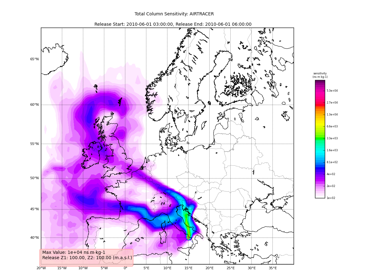
This is redundant data to the grid, and will likely change in future versions of reflexible. However, the important point to note is that the 0th element is the Total Column.
Using the plotting tools of reflexible we can plot the total column easily:
In [61]: rf.plot_totalcolumn(H, myc.total_column, map_region='NorthAtlantic')
This should return an image similar to:
Adding Trajectories
I use the read_trajectories() function to read the trajectories.txt
file and get the trajectories from the run output directory.:
T = rf.read_trajectories(H)
Note, that the only required parameter is the Header “H”, this provides all the metadata for the function to read the trajectories. This is a function that accepts simply the “H” instance or a path to a trajectories file.
Now we can see how we might batch process a backward run and create
total column plots as well as add the trajectory information to the
plots. The following lines plot the data sets using the
plot_totalcolumn(), plot_trajectory(), and
plot_footprint().
Warning
There is a lot of reliance on the mapping module in the plot_routines. If you
have problems, see the mapping.py file. Or the mapping
docstrings. Documentation of this module is presently incomplete but I
am working on it.
In order to reuse figures which is much faster when working with the basemap module, I create a “None” objects for passing the figure instances around:
TC = None
After that we loop over the keys (s=species, and k=rel_i) of the H.C
attribute we created by calling fill_backward. Note, I named this
attribute C for “Cumulative”. In each iteration, for a new
combination of s,k we pull the data object out of the dictionary. The
“data” object is returned from the function readgridV8() and has
some attributes that we can use later in conjunction with the
plot_totalcolumn() function and for saving and naming the
figures. See for example the following lines:
for s, k in H.C:
    data = H.C[(s, k)]
    TC = rf.plot_totalcolumn(H, data, map_region='Europe', FIGURE=TC)
    TC = rf.plot_trajectory(H, T, k, FIGURE=TC)
    filename = '%s_tc_%s.png' % (data.species, data.timestamp)
    TC.fig.savefig(filename)
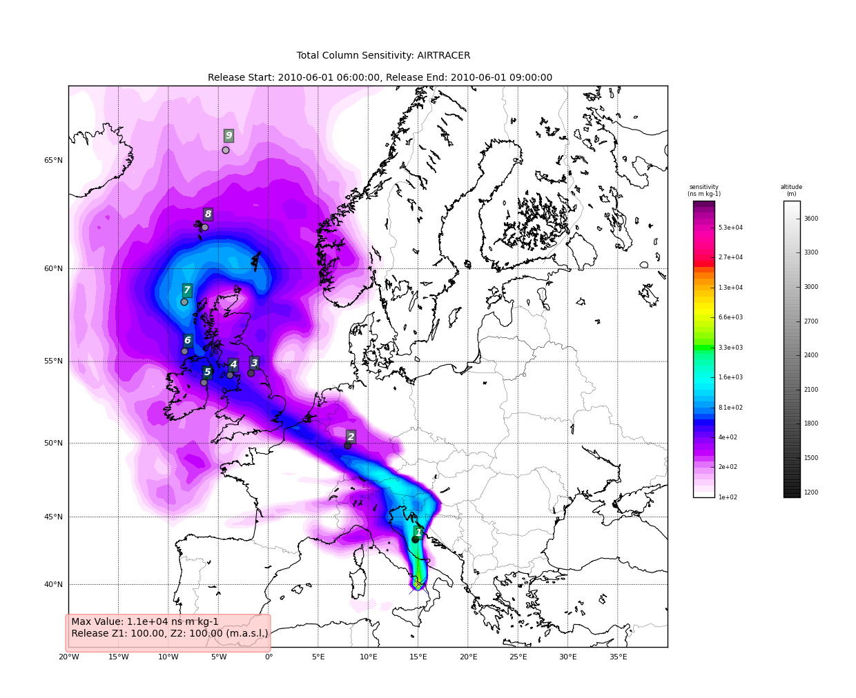
This will create filenames based on the data metadata and save the figure to the path defined by filename. You should now have several images looking like this:
The next step is the use the source and learn more about the functionality of the module. I highly recommend the Ipython interpreter and use of the Tab key to explore the modules methods.
Enjoy!